3.7.1 Fields

Content 

• Concept of a force field as a region in which a body experiences a non-contact force.
• Students should recognise that a force field can be represented as a vector, the direction of which must be determined by inspection.
• Force fields arise from the interaction of mass, of static charge, and between moving charges.
• Similarities and differences between gravitational and electrostatic forces:
• Similarities: Both have inverse-square force laws that have many characteristics in common, eg use of field lines, use of potential concept, equipotential surfaces etc.
• Differences: masses always attract, but charges may attract or repel.

Concept of a force field as a region in which a body experiences a non-contact force.

The definition of a force field is a region in which a body experiences a non-contact force; an example is the gravitational field.

Students should recognise that a force field can be represented as a vector, the direction of which must be determined by inspection.

A force field can be represented by vectors. We can represent a gravitational force field by lines directed towards the attracting body, the Earth for example. The field lines point along the direction the force acts. Also, we must define the field line directions for a positive and negative charge. We define a positive charge as a “source” of charge (for reasons that will become clear in a first year vector calculus course), thus the field lines emanate out from a positive charge. Contrarily, for a negative charge, we define the field lines to be directed into the charge. Again, these are purely a convention, just as the direction an electric current moves around a circuit is too, purely a convention; choosing the opposite directions would not change the nature of our results.

Force fields arise from the interaction of mass, of static charge, and between moving charges.

The interaction of mass is facilitated by the gravitational field. The electric field facilitates the interaction of static charge. For moving charges, the interaction is somewhat more complicated to state, but force fields will also arise from the interaction between moving charges.

Similarities and differences between gravitational and electrostatic forces:

Similarities:

• Both force laws follow an inverse-square relation
• Both use the “potential” concept. The potential at a point is actually an intrinsic part of the field, and directly relates to the strength of an electric field. This will be covered further in the first year undergraduate Electricity and Magnetism course.
• Both make use of field lines to indicate strength of field, and direction the field acts.
• Both have associated equipotential surfaces – surfaces that your potential remains constant over. Thus work done moving over an equipotential surface is 0J.

Differences are that masses will always attract; however charges may attract or repel depending on whether they are like charges or not.

• The gravitational force is always attractive, because masses always attract each other. Whereas, the electrostatic force can be attractive or repulsive, thus the electrostatic force can be negative or positive. It will be positive (repulsive) between like charges, and negative (attractive) between unlike charges.

3.7.2 Gravitational Fields

3.7.2.1 Newton’s law

Content

• Gravity as a universal attractive force acting between all matter.
• Magnitude of force between point masses:  where G is the gravitational constant.

Gravity as a universal attractive force acting between all matter.

Gravity is a universal attractive force that acts between all matter (mass). Our first mathematically rigorous description of gravity came from Sir Isaac Newton, this description was furthered and refined by Albert Einstein in the early 1900s. Interestingly, Albert Einstein’s so called general theory of relativity only makes corrections on the order of 10^-15. So despite primitive in nature, Isaac Newtons formulation of our universe is no less remarkable.

Magnitude of force between point masses: where G is the gravitational constant 

F = Gm₁m₂/r² is the equation that enables you to calculate the magnitude of the force acting between point masses. It is important to remember that this calculates the magnitude of the attractive force acting between point masses. By virtue of the attractive nature of gravity, this equation should have a negative sign present, but since we are interested in the magnitude – that is the absolute value – we ignore the sign of the force.

The value of G is given in the equation sheet, and is 6.67 x 10^-11 Nm²kg^-2. The ‘r’ is the distance between the centre of mass of the two objects – IT IS NOT THE DISTANCE BETWEEN THE SURFACES OF THE TWO OBJECTS, that’s important to remember… Hence, for a particle on the surface of the Earth ‘r’ will be approximately 6.4 x 10⁶ m, as this is the distance from the centre of the Earth to its surface (definitely not 0m). Usually the equation will be written using ‘Mm’ where the ‘M’ will be the larger mass, the one ‘doing the attracting’ e.g. the Sun in a question involving the Sun and Earth.

AQA June 2010 Unit 4 Section B Q1a

Question:

State Newton’s law of gravitation

Answer:

• Force of attraction between two point masses
• Proportional to product of masses
• Inversely proportional to square of distance between them

3.7.2.2 Gravitational field strength

Content:

• Representation of a gravitational field by gravitational field lines.
• g as force per unit mass as defined by g = F/m.
• Magnitude of g in a radial field given by g = GM/r².

Representation of a gravitational field by gravitational field lines.

We can represent the gravitational field using gravitational field lines. This is convenient as it allows us to identify how the gravitational field strength varies, if at all.

The figure shown below illustrates a radial field. Radial means to diverge or spread from a common point. Clearly the below diagram is a schematic – we could draw more lines radiating from the mass, but it won’t help us much. From this diagram we can see that the field strength decreases as you move away from the mass. We know this because the field lines become less dense i.e. per area of space there are less field lines contained.

This figure shows a uniform field. We can see its uniform because the field lines remain a constant distance from each other as you move from the surface that they originate from: a uniform field means a constant field strength. In fact the surface of the Earth can be approximated as behaving as a uniform field, i.e. the gravitational field strength, g, on the surface of the Earth, is a constant. 

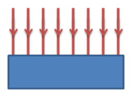
g as force per unit mass as defined by g = F/m (in a uniform field).

The gravitational field strength, g, is calculated (in a uniform field) using the following relationship: g = F/m. As you move vertically upwards from the surface of the Earth the attraction F, between you and the Earth, will decrease: we can see this directly from the equation F = GMm/r². However, for small distances above the surface of the Earth the force F will not change by much. Therefore if we moved a 1kg mass 25m vertically upwards from the surface of the Earth, the force acting on it can be approximated as constant. Therefore, the gravitational field strength is said to be constant because clearly our mass does not change.

Magnitude of g in a radial field given by g = GM/r².

Generally speaking the gravitational field is not a uniform field because it radiates outwards from masses, so field lines become less densely populated, thus field strength is weaker. This means we require a relation that will give us the value of the gravitational field strength due to a non uniform field. Conveniently we are given it: g = GM/r²

Remember that g is the gravitational field strength, G is the gravitational constant, M is the mass of the attracting body, and r is the radial distance from the centre of the planet.

3.7.2.3 Gravitational potential

Content

• Understanding of definition of gravitational potential, including zero value at infinity
• Understanding of gravitational potential difference.
• Work done in moving a mass m given by ΔW = mΔV
• Equipotential surfaces.
• Idea that no work is done when moving along an equipotential surface.
• V in a radial field given by V = – GM/r.
• Significance of negative sign.
• Graphical representations of variations of g and V with r.
• V related to g by: g = – ΔV/Δr
• DV from area under graph of g against r.

Opportunities for Skills Development

• Students use graphical representations to investigate relationships between v, r and g.

Understanding of definition of gravitational potential, including zero value at infinity.

Gravitational potential: is the work done per unit mass to move a test mass from infinity to that point. REMEMBER: GRAVITATIONAL POTENTIAL RELATES TO ENERGY!

It is a very, very important quantity. In fact it is fundamental in our picture of gravity, electrostatics, and any field representation for that matter. ‘Potential’, whether it be in the context of gravity, electricity, magnetism is FUNDAMENTAL. Just like forces and accelerations are fundamental in our Newtonian view of the world, gravitational potential is fundamental in our view of fields. Think hard about what I write here, and if what I say does not become clear now, it will become clear in your first year electricity and magnetism course. Gravitational potential is a property of the gravitational field. OK, it is an inherent property of the field. It is defined uniquely everywhere in the universe, irrespective of whether a mass rests there or not. We can use it to find the force acting at a point. It gives us information about the field, without requiring objects in the field to make some analysis or prediction. Anyway, the take home message is that gravitational potential is important, and if you are faced with question about a gravitational field, you should think POTENTIAL first.

Moving on, we MUST always define gravitational potential relative to another potential – remember that. This is why we define gravitational potential at a point – for example at the surface of the Earth – relative to infinity. Why infinity? Well because we can say that at infinity gravitational potential = 0, this makes calculations far more convenient. It turns out to be far more convenient than defining the Earth as being at 0 potential, for instance.

There is one possible conceptual difficulty with this way of defining potential. Think about this:

If I move from the Earth to infinity (1000000000… miles away), clearly I need to do work to get there. So to be clear, I must do work to move from a point on the surface of the Earth to infinity, the point in space where gravitational potential is defined as being equal to 0. You might think that this must mean we start off with negative gravitational potential, and you would be absolutely correct.

The Earth’s surface has a gravitational potential of -63MJkg^-1. This means that to move a 1kg mass from the surface of the Earth to infinity, we must do 63MJ of work (energy). If we had a 2kg mass we would require 126MJ, 3kg 189MJ and so on.

Understanding of gravitational potential difference.

The gravitational potential difference is the difference in potential between two points in a gravitational field. The gravitational potential on the surface of the Earth is around -63MJkg^-1 and at another point 1000km above the surface of the Earth is approximately -54MJkg^-1. Therefore the gravitational potential difference is -54-(-63) = 9MJkg^-1.

From this we can deduce that, to move a 1kg mass 1000m vertically upwards from the surface of the Earth requires 9MJ of energy. So if you are given a question, and given only the gravitational potential at two points, you could find the energy an arbitrary (randomly chosen valued) mass would require to move between those two points.

Work done in moving a mass m given by ΔW = mΔV.

Recall we defined gravitational potential as the work done per unit mass to move that mass from infinity to a point in space. Our equation follows from this, ΔV = ΔW/m where ΔV is the change in gravitational potential, ΔW is the work done (the change in gravitational potential energy) and m is the mass. Don’t be confused by ‘ΔV’, Δ only means change in. And of course it is going to be there, gravitational potential changes at every point in space. We can rearrange ΔV = ΔW/m to give the equation written in the above heading.

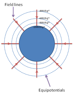
Equipotential surfaces.

In fact, I may have told a little lie above. Gravitational potential does not change when you move along surfaces called equipotential surfaces.

Equipotential surface: a surface whereby on which no work is done when moved along. This is because the gravitational potential at these equipotential surfaces is the same the whole way along, so in the equation ΔW = mΔV, the change in gravitational potential (ΔV) is 0, so work done is 0. The diagram below shows equipotential surfaces.

 

Idea that no work is done when moving along an equipotential surface.

To reiterate, no work is done when you move along equipotential surfaces.

V in a radial field given by V = – GM/r.

To calculate the gravitational potential in a radial field you use the equation given above. G = gravitational constant given in the equation sheet, M is mass, for example mass of the Earth. r is the distance from the centre of the object. The M in the equation will always be the mass of the object responsible for the gravitational attraction.

Significance of negative sign.

The negative sign indicates that gravity is an attractive force, pulling objects together.

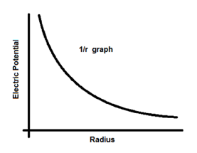
Graphical representations of variations of g and V with r.

 

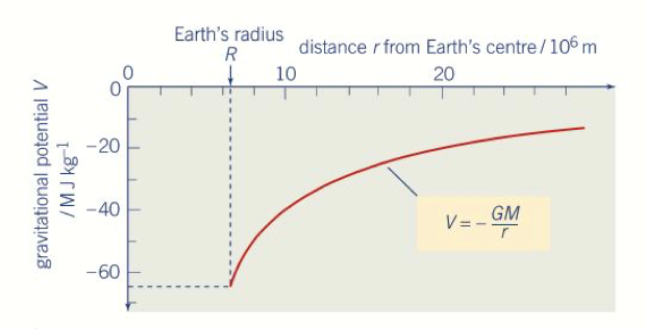
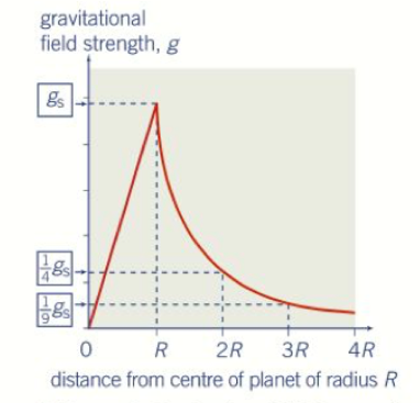
Since g = GM/r², it can be said that g  1/r². This gives the shape of the graph that you can see. However, when moving towards the centre of a planet, the gravitational field strength reduces linearly from g to 0. On the other contrary, V = -GM/r, so it can be said that V  1/r, to give the shape of the graph shown above.

V related to g by: g = – ΔV/Δr.

The gravitational field strength can also be calculated from the potential gradient, where g = – ΔV/Δr. It can also be looked at as the change in potential per metre at a point, near the surface of the Earth a 1kg mass gains 9.81J of energy per metre it is raised, but this becomes less the further from the surface of the Earth that you move.

V from area under graph of g against r.

The change in potential can be found by calculating the area under a graph of g against r.

3.7.2.4 Orbits of planets and satellites

Content

• Orbital period and speed related to radius of orbit; derivation of T² ∝ R³
• Energy considerations for an orbiting satellite.
• Total energy of an orbiting satellite.
• Escape velocity.
• Synchronous orbits.
• Use of satellites in low orbits and geostationary orbits, to include plane and radius of geostationary orbit.

Opportunities for Skills Development

• Estimate various parameters of planetary orbits, eg kinetic energy of a planet in orbit.
• Use logarithmic plots to show relationships between T and r for given data.

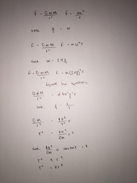
Orbital period and speed related to radius of circular orbit; derivation of T² ∝ R³

Kepler’s Third Law states that the orbital period is related to the radius of the circular orbit where T² ∝ R³. The picture below shows the derivation of Kepler’s Law.

 

Energy considerations for an orbiting satellite.

An orbiting satellite will possess both kinetic energy and gravitational potential energy. Its kinetic energy will be as a result of its velocity and mass, and its gravitational potential energy will be as a result of its position in the gravitational field as well as its mass. If a satellite moved closer to the Earth, it would lose gravitational potential energy, so this energy must be converted to kinetic energy. Thus the orbital time of the satellite would decrease as its kinetic energy would increase thus its velocity also.

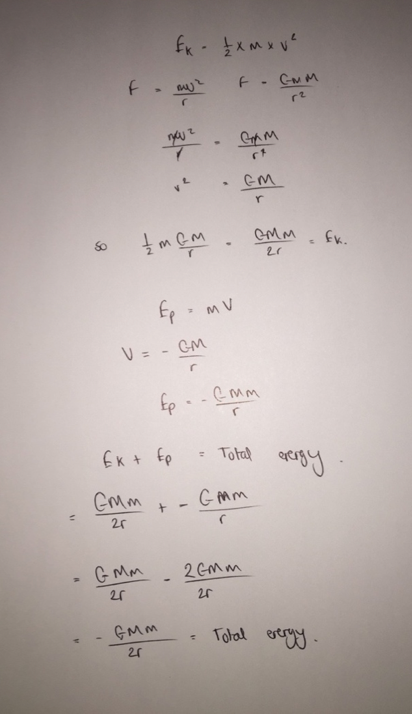
Total energy of an orbiting satellite.

In order to calculate the kinetic energy of satellite we use , so we need to calculate the velocity of the satellite. In order to do this, we need an equation with v in, so we can use F = mv²/r. However if we do not have all of the information that we need to solve v, you can equate the equations F = mv²/r and F = GmM/r². The result of this when you solve for the velocity is v² = GM/r So if we substitute this into  we end up with GmM/2r. Now we have an equation for the kinetic energy we need to find one for the gravitational potential energy. Gravitational potential is equal to V = – GM/r, so to find its gravitational potential energy at this point we must multiply by m. This gives us – GMm/r  , so when we do E_k + E_p as shown below, we are left with – GMm/2r

 

Synchronous orbits.

A synchronous orbit is defined as “an orbit in which an orbiting body (usually a satellite) has a period equal to the average rotational period of the body being orbited (usually a planet), and in the same direction of rotation as that body.”  This type of orbit is also referred to as geosynchronous. This type of orbit can have any inclination and eccentricity, that is, it can be tilted with respect to the poles of the earth and it may not be a circular orbit.

Use of satellites in low orbits and geostationary orbits, to include plane and radius of geostationary orbit.

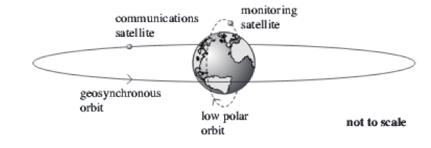
A synchronous orbit is defined in the previous topic. There is however, a special type of synchronous orbit, called a geostationary orbit. A geostationary orbit is a geosynchronous orbit that occurs around the equator of the Earth. It orbits at 35,786 km above the surface of the Earth, thus the radius of its orbit is roughly 4.2 x 10⁷m (this is 35786 km added to the radius of the Earth: 6400 km). This special case of geosynchronous orbit is unique as an observer from Earth would appear to see a satellite in geostationary orbit in the same position, all day, every day. It can be said that every geostationary orbit is also geosynchronous, but not the other way around. The diagram below illustrates the special case of geosynchronous orbit, and also shows a different type of geosynchronous orbit.

Low polar orbits are also shown below; these orbits are not geosynchronous as they do not have the same orbital time period as the Earth. Since their radius is smaller, and T² ∝ R³, then the time period must also be much shorter, so they are useful as satellites to monitor changing conditions on Earth, whereas the geostationary orbit is more useful for communication.

 

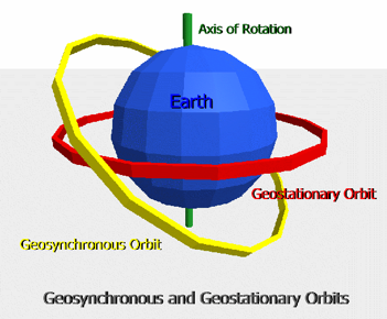
Geosynchronous orbit above Equator (Geostationary):

• Its orbital period matches the Earth’s rotational period exactly (roughly 24 hours).
• A satellite in geosynchronous orbit will maintain the same position relative to the Earth.
• There is only one type of orbital radius possible.
• A satellite will travel west to east above the Equator (the same direction as the Earth’s rotation).
• The orbital height is higher than a polar orbit satellite.
• The speed is much less than a satellite in polar orbit.
• It will scan a restricted, and fixed area of the Earth’s surface only, due to its orbit.
• Its applications are usually in telecommunications, so cable and satellite TV, radio and other digital information.
• The satellite is in continuous contact with the receiving or transmitting aerial as its position is maintained relative to the Earth, thus aerials can be in fixed positions.
• You do need a higher signal strength than that of a polar satellite as its height above the surface of the earth is much greater.

Low Polar Orbit

• It usually has an orbital period of only a few hours.
• The Earth rotates relative to the orbit of a satellite in low polar orbit,
• You are able to get many orbits with different radii and periods.
• Much lower orbital height than geosynchronous.
• The speed of satellites in low polar orbit is much greater than that of one in a synchronous orbit.
• Its main applications are in surveillance on Earth i.e. mapping, weather observations or environmental monitoring.
• It enables access to every point on the Earth’s surface every day.
• You can collect data from places inaccessible to humans.
• The contact with the transmitting or receiving aerial is intermittent as the Earth moves relative to the orbit of a satellite in low polar orbit.
• An aerial would require a tracking facility.
• You would require a lower signal strength than a synchronous satellite.

3.7.3 Electric Fields

3.7.3.1 Coulomb’s law

Content

• Force between point charges in a vacuum: 
• Permittivity of free space, e₀.
• Appreciation that air can be treated as a vacuum when calculating force between charges.
• For a charged sphere, charge may be considered to be at the centre.
• Comparison of magnitude of gravitational and electrostatic forces between subatomic particles.

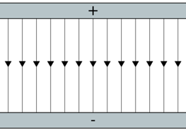
Force between point charges in a vacuum:

The force between point charges follows similar rules as the force between two masses, where the force is proportional to the product of the two charges, and inversely proportional to the square of their distance apart.

Permittivity of free space, e₀.

The permittivity of free space is given by the symbol e₀, and has the value of 8.85 x 10^-12. It is basically the permittivity of a vacuum, and is given to you in the equation sheet.

Appreciation that air can be treated as a vacuum when calculating force between charges.

Since the force between point charges is for a vacuum, in questions we can assume that air is a vacuum.

For a charged sphere, charge may be considered to be at the centre.

Comparison of magnitude of gravitational and electrostatic forces between subatomic particles.

The electrostatic force between subatomic particles is far greater than the gravitational attraction between them. For example, if you hold two electrons 1m apart from each other, the gravitational attraction between them will be F = G x (9.11×10^-31)² / 1², which equals around 5.5 x 10^-71 N. The electrostatic force of repulsion will be equal to 1/4πe₀ x (-1.6 x 10^-19)²/ 1², which equals around 2.3 x 10^-28 N. Therefore, the electrostatic force divided by the gravitational force equals 4 x 10⁴². This means the electrostatic force is 4 x 10⁴² times bigger, so the gravitational force is pretty much negligible when dealing with subatomic particles.

3.7.3.2 Electric Field strength

Content

• Representation of electric fields by electric field lines.
• Electric field strength.
• E as force per unit charge defined by E = F/Q
• Magnitude of E in a uniform field given by E = V/d
• Derivation from work done moving charge between plates: Fd = QΔV
• Trajectory of moving charged particle entering a uniform electric field initially at right angles.
• Magnitude of E in a radial field given by 

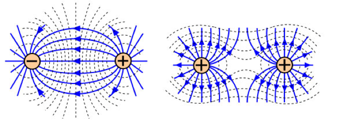
Representation of electric fields by electric field lines.

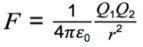
Since charges can be positive and negative, you will get different electric field lines depending on this factor.

For a positive charge its electric field lines will look as follows:

 

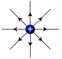
For a negative charge its electric field lines will look as follows:

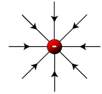
These fields are radial fields, just like the radial field you will get in gravitational fields. It is also possible to get a uniform field. In a uniform field i.e. between two plates, the field will look as follows.

You will also see different electric field line when two charges interact with each other.

Electric field strength. E as force per unit charge defined by E = F/Q

Electric field strength is the force per unit charge acting on a positive test charge placed at that point. As an equation it is: E = F/Q, and has the unit NC^-1 or Vm^-1. Electric field strength is a vector quantity, so if two charges are interacting, you may be asked to find the resultant electric field.  By convention, the electric field points in the direction that a positive charge placed at that point in the field would feel a force.

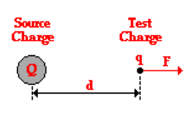
The electric field strength at a distance d from the source charge Q, would be E = F/q. Since it is the force per unit charge acting on a positive test charge placed at that point, the charge used is therefore the charge on the test charge (q), not the source charge (Q).

The electric field strength is not actually dependent upon the quantity of the charge on the test charge. The electric field strength at any given location around the source charge Q will be measured to be the same regardless of what test charge is used. This is because if you increase the charge on the test charge by a factor of say, 2, then according to Coulomb’s Law, this increase in charge will be accompanied by an increase in the force. The increase in force would be by the same factor, so the denominator and numerator in E=F/Q would always increase by the same factor, thus electric field strength at any given point would be constant regardless of the charges.

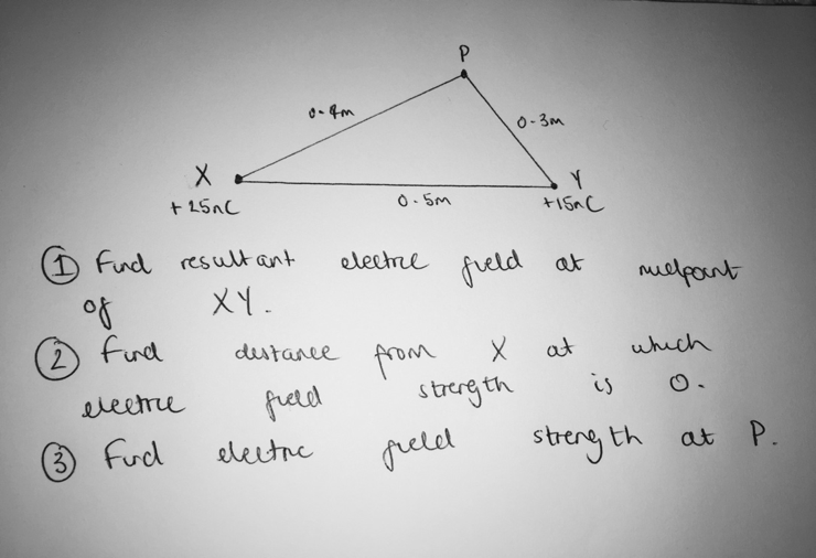
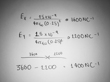
• To find the resultant electric field from X and Y, we must first find the magnitude of the electric field strength from each of them. Electric field strength, E, can be calculated by using E = Q/4πe₀r². The picture below shows how to approach this question. You must first work out the electric field from X (E_X) and then from Y (E_Y). Since electric field strength is a vector, and these two fields are working in opposite directions, the magnitude of the resultant is 3600 – 2200 = 1400NC^-1. Therefore, this is the electric field strength at the mid-point of XY.

• We know that at a distance we can call d, the electric field strength is 0. Since the remaining distance must be (0.5 – d), so we can place this onto the diagram.

Then if we make the electric field strength at that distance from X equal to the electric field strength at that distance from Y, and solve to find d, we get 0.28m from X.

• First we must calculate the electric field at P due to X and then due to Y. These electric fields are not acting in the same direction (their directions are shown on the diagram), and since they are vectors we can use the head to tail method for vectors to find the resultant electric field. Also to link back to the definition of an electric field, the direction of these vectors is the direction that a positive test charge placed at P would feel a force. Using this method, we construct a right angled triangle and can use Pythagoras to solve for the resultant electric field.

Magnitude of E in a uniform field given by E = V/d.

In a uniform field, the electric field strength is given by the potential difference between two plates, divided by their distance apart.  So if the potential difference were 10V and the distance were 1m, the electric field strength would be 1Vm^-1/NC^-1.

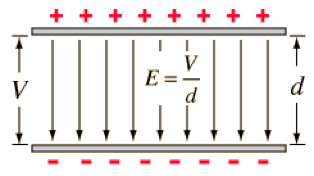
Since E = F/Q, then F/Q = ΔV/d, therefore Fd = QΔV. The force multiplied by the distance is equal to the work done, so the charge multiplied by the change in potential difference is equal to the work done.

Trajectory of moving charged particle entering a uniform electric field initially at right angles.

If a positively charged particle enters a uniform electric field initially travelling perpendicular to the field, then it will accelerate uniformly in the direction of the field and move in a parabolic fashion. For a negatively charged particle i.e. an electron, it would move in the opposite direction to the electric field as it is repelled by the negative plate.

In the question below we have an electron entering a uniform field between two plates 1m apart, travelling perpendicular to the direction of the field. The question is to find the vertical distance moved by the electron in 0.5ms, and which direction the electron moves in.

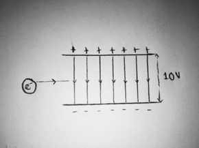
The electron is clearly going to move towards the positive charge, in a parabolic direction upwards. To find the vertical distance moved by the electron we need to find what its acceleration is. For acceleration we can use F = ma, and also F = EQ. First of all we need to know the electric field strength within the uniform field, which is given by E = V/d, so equal to 10/1 = 10Vm^-1. Now we have the electric field strength we can find the force acting on the electron, equal to F = EQ, so 10 x 1.6 x 10^-19. This value of F can be used now to find the acceleration using F = ma. So this value of F calculated previously (1.6 x 10^-18), can be divided by the mass of the electron (9.11 x 10^-31) to give the acceleration of the electron. This acceleration is equal to 1.75 x 10¹² ms^-2.

Now we have the acceleration of the electron, we can use the suvat equations to find the vertical distance moved. The information that we have is u = 0 as the electron is initially moving perpendicular to the direction of the field with no vertical velocity. We also now know a = 1.75 x 10¹² ms^-2, and we want to find the distance travelled in 0.5ms (0.5 x 10^-6s). Using s = ut + at²/2 we can obtain a value of s equal to 0.22m.

If asked to find the horizontal distance travelled by the electron we would need to know its initial velocity, and assuming that the acceleration horizontally is 0, it would be possible to obtain a value for the horizontal distance travelled in a given time.

Magnitude of E in a radial field given by E = 1/4πe₀ x Q/r².

The equation above can also be written as E = Q/4πe₀r². This is the value of E in a radial field, and can be derived from the fact that E = F/q, so using Coulomb’s Law that F = qQ/4πe₀r². We can substitute this equation in for F, and when you divide it by q, you get E = Q/4πe₀r². 

3.7.3.3 Electric potential

Content

• Understanding of definition of absolute electric potential, including zero value at infinity, and of electric potential difference.
• Work done in moving charge Q given by ΔW = QΔV
• Equipotential surfaces.
• No work done moving charge along an equipotential surface.
• Magnitude of V in a radial field given by 
• Graphical representations of variations of E with V and r.
• V related to E by E = ΔV/Δr
• ΔV from area under graph of E against r.

Understanding of definition of absolute electric potential, including zero value at infinity, and of electric potential difference.

Absolute electric potential means that it is not relative, and means the amount of electric potential that a point has is the same irrespective of charge. Electric potential is the work done per unit positive charge on moving a small positive test charge from infinity to that point. Electric potential is a scalar quantity, so the electric potential at one point due to two different charges will add up. Thus the electric potential at an equidistant point of 40mm from two different charges will be the sum of their electric potentials.

Because of the existence of repulsion, it is possible to obtain positive and negative potential energy values. If you were to bring a positive test charge from infinity towards another positive source charge, there would be a repulsion between the charges, so we must do work to move the test charge towards the source charge. This work is stored as electric potential energy of the test charge. This concept would also apply to two negative charges. Although in both cases the potential energy of the test charge increases (from 0) as it approaches the source charge. Therefore the electric potential of the test charge is positive. However if you had a test charge and source charge of opposite signs, they will attract each other. This means it now takes work to separate the two charges, which is stored as electric potential energy in the test charge. This energy on the test charge will increase towards 0 as their separation increases, so the test charge must have a negative potential energy.

Work done in moving charge Q given by ΔW = QΔV.

The work done in moving a charge Q, is given by multiplying the charge by the change in potential over a given distance. So if a 10C charge is moved across a potential of 10V, the work done would be 100J.

Equipotential surfaces.

Equipotential surfaces are surfaces whereby the electric potential does not change. These equipotential surfaces are similar to the equipotential surfaces of the gravitational field. The diagram below shows different equipotential lines around like charges and unlike charges.

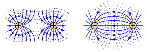
Since electric potential is a scalar quantity, the potential at a given point will add up. For unlike charges shown, the electric potential at the middle will cancel out, hence the vertical equipotential line separating the two charges.

No work done moving charge along an equipotential surface.

In the equation for work done ΔW = QΔV, the ΔV is significant as this is the change in potential. When moving over an equipotential surface, your electric potential will not change, so ΔV = 0, thus ΔW = 0.

Magnitude of V in a radial field given by

Calculating V in a radial field is done by using the equation above.

Graphical representations of variations of E with V and r.

Since electric field strength is proportional to 1/r², and electric potential is proportional to 1/r, the graphs will look similar but have a slight difference.

The graph of electric field strength against r would be different in that it would decrease at a faster rate since electric field strength would decrease by 1/r² as opposed to 1/r.

V related to E by E = ΔV/Δr.

The electric field strength at a point is equal to the change in potential divided by the change in distance between the charges. This is proven by the fact that electric potential equals Q/4πe₀r, so if you divided by r you will get Q/4πe₀r², which is equal to the electric field strength. Thus if you have an electric field strength you can multiply it by the change in distance to get the electric potential.

3.7.4 Capacitance

Content

• Definition of capacitance: C = Q/V

Definition of capacitance: C = Q/V

Capacitors are designed to store charge, and you can make a capacitor by placing to nearby metal plates parallel to each other. One plate is positive and one negative, with an equal and opposite charge. The equation to calculate capacitance is C = Q/V, where C is capacitance units Farads (F), Q is the charge in Coulombs (C) and V is potential difference between the plates (V).

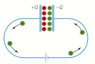
The two metal plates are insulated from each other, and in the capacitor electrons move from the positive terminal to the negative terminal. This explains the loss of charge on the positive end being equal to the gain in charge at the negative terminal.

3.7.4.3 Parallel Plate Capacitor

Content

• Dielectric action in a capacitor C = Aε_rε₀/d.
• Relative permittivity and dielectric constant
• Students should be able to describe the action of a simple polar molecule that rotates in the presence of an electric field

Opportunities for Skills Development

• Determine the relative permittivity of a dielectric using a parallel-plate capacitor.
• Investigate the relationship between C and the dimensions of a parallel-plate capacitor eg using a capacitance meter.

Dielectric action in a capacitor C = Aε_rε₀ /d.

To store more charge on the plates of a capacitor, an electrically insulating dielectric can be put in between them. The presence of a dielectric will reduce the effective electric field as when placed between two metal plates, it will produce an electric field in the opposing direction to the field of the charges on the plate. The equation for calculating capacitance in a dielectric is C = Ae₀e_r/d, where C is capacitance (F), A is cross sectional area (m²), ε₀ is permittivity of free space and ε_r  is relative permittivity, and d is the distance between parallel plates.

A material may contain polar molecules, and if so, they are usually arranged randomly in the absence of an electric field. Applying an electric field will polarise the molecules in material as shown below.

This means that one surface will gain positive charge and one will gain negative charge, i.e. the side of the dielectric that faces the positive plate will gain more negative charge. In dielectric materials that are already polarised, but face in opposite directions, when placed in a parallel plate capacitor the molecules will be attracted towards the positive plate due to the negatively charged electrons.

The resultant effect of the dielectric is that more charge can be stored, where the surface of the dielectric by the positive plate will gain negative charge, and negative plate positive charge. The positive end on the dielectric will draw more electrons onto the negative plate, then the negative side will repel electrons back to the battery from the positive plate.

Since Q/V = C, then if Q increases C will also increase, so in conclusion, the effect of a dielectric in a circuit is to store more charge in a capacitor for a given potential difference, so increase the capacitance.

Relative permittivity and dielectric constant

Relative permittivity the ratio of charge stored with a dielectric to that without a dielectric, where ε_r = Q/Q₀, also equal to C/C₀, ε_rε₀ or even I/I_0. It has no units because ultimately it is a ratio of permittivity’s. The relative permittivity is also referred to as the dielectric constant, and the values of dielectric constants range from values like 2.3, to 81 for water.

Students should be able to describe the action of a simple polar molecule that rotates in the presence of an electric field

In alternating electric fields, polar dipoles will rotate as the electric field constantly changes direction. Non-polar dipoles will oscillate in one direction and then the opposite direction.

3.7.4.3 Energy stored by a capacitor

Content

• Interpretation of the area under a graph of charge against pd. E = QV = CV² =  Q/C²

Interpretation of the area under a graph of charge against pd. E = QV/2 = CV²/2 =  Q/2C²  

Energy is stored as electric potential energy in a capacitor, and the amount of energy stored in a capacitor can be calculate from the area under a graph of charge against potential difference. Since work done is equal to the voltage multiplied by charge (W=QV), then for a capacitor energy stored, E will be equal to  QV as from a graph of Q against V (straight line), this would be the area underneath.

3.7.4.4 Capacitor charge and discharge

Content

• Graphical representation of charging and discharging of capacitors through resistors. Corresponding graphs for Q, V and I against time for charging and discharging.
• Interpretation of gradients and areas under graphs where appropriate.
• Time constant RC
• Calculation of time constants including their determination from graphical data.
• Time to halve, T_1/2 = 0.69RC
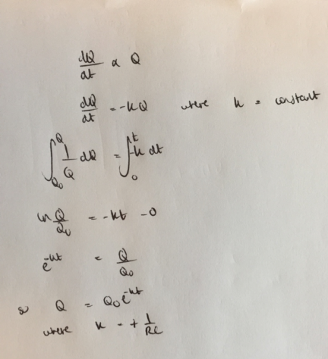
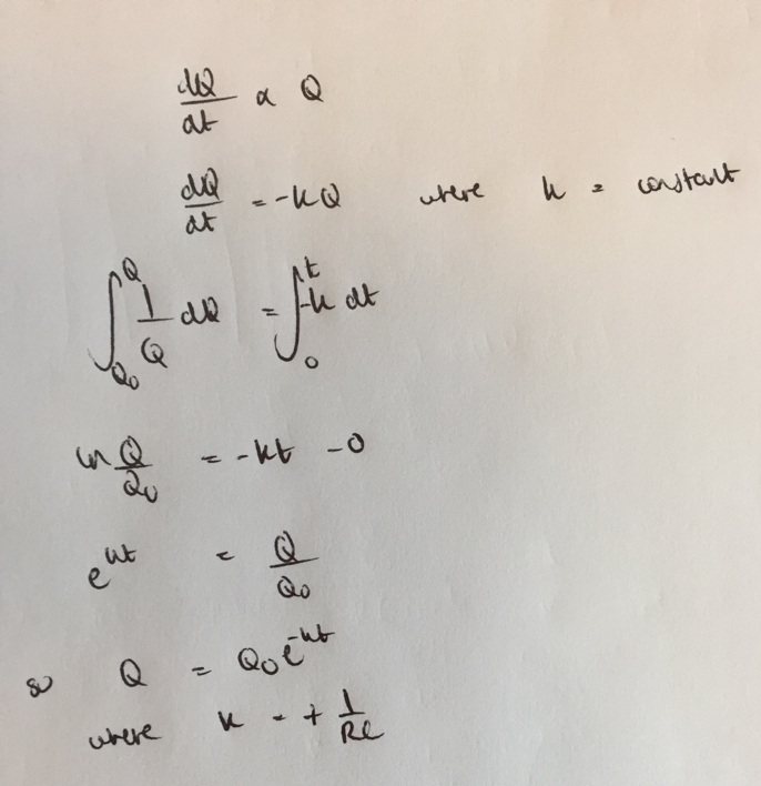
• Quantitative treatment of capacitor discharging, Q = Q₀e^-t/RC
• Use of the corresponding equations for V and I
• Quantitative treatment of capacitor charge, Q = Q₀(1-e^-t/RC)

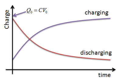
Graphical representation of charging and discharging of capacitors through resistors. Corresponding graphs for Q, V and I against time for charging and discharging.

The graph for charge against time for charging and discharging is shown below on the left, the two lines would be the same if the graph were voltage against time. To the right we have current against time, which is the same for charging or discharging.

Discharging a capacitor through a fixed resistor

In this process current will decrease quicker at first, and then more gradually to zero. The current decrease like this because the potential difference decreases across the capacitor as it loses charge, and I = V/R where R is constant. Moreover, this graph shows that the current will decrease exponentially with time, and thus according to the equation I = I₀e^-t/RC.  This means that after a time t = RC (RC is covered under the next heading), I = 0.37I₀, so the current decreases by approximately 63% of its original value. The same principle applies in the cases of both charge and potential difference.

Charging a capacitor through a fixed resistor

The graph showing the charging of a capacitor for current is identical to the graph showing discharging. The current in the circuit will begin high as there is a larger rate of flow of charge, then this rate of flow will decrease progressively throughout time. However according to the graph charge increases exponentially with time, and so too does the potential difference.

Interpretation of gradients and areas under graphs where appropriate

The gradient of charge-time is current, because I = ΔQ/Δt.

The area under a current-time graph is equal to the amount of charge stored on the plates of the capacitor as we know the equation Q = It.

We also know that the area under a voltage-time graph is equal to the energy stored in the capacitor, so E = 1/2QV. We know this because W=E=QV. This means that half of the energy is wasted as a result of resistance to the flow of charge in the circuit. This energy is then transferred to the surroundings as thermal energy for example.

Other relationships can be formed between equations, and the gradients/area under of graphs can be determined using the equations governing capacitance. For example, the area under a graph of capacitance against voltage squared, will also yield the energy stored in the capacitor, equal to 1/2CV². However, the listed relationships above are the main ones.

Time constant RC

The time constant is equal to the resistance multiplied by the capacitance, and the units are in seconds, which can be derived from the units of resistance and capacitance. If the time constant, RC, was 6 seconds in a circuit, then after 6 seconds the charge will have fallen to 63% its original value. Because Q = Qe^-1.

Calculation of time constants including their determination from graphical data.

Take for instance a graph of charge-time for the discharging of a capacitor. Say the maximum value was 1C and found the time that it took for the charge to fall from 1C to 0.37C, this time that you found would be equal to the time constant of the circuit. This is because according to Q = Q₀e^-t/RC, Q = 1e^-1 » 0.37C. From knowing this value of the time constant, for example if it were 6s, you could calculate the resistance/capacitance of the circuit. This is because you know that 6 = RC = time constant, so 6/C = R and 6/R = C.

Time to halve, T_1/2 = 0.69RC

If you were to substitute t » 0.69RC into Q = Q₀e^-t/RC, you would get Q = Q₀e^-0.69 because 0.69RC/RC = 0.69. And the result of this is Q » 0.5Q₀. This means that after a time equal to 0.69RC, the charge falls to approximately half of its original value.

Quantitative treatment of capacitor discharging, Q = Q₀e^-t/RC

The discharging of a capacitor is modelled by the equation Q = Q₀e^-t/RC. This equation also explains the exponential decrease on a charge – time and a voltage – time graph for the discharging of a capacitor.

Use of the corresponding equations for V and I

Quantitative treatment of capacitor charge, Q = Q₀(1-e^-t/RC)

The capacitor charges exponentially too, and is modelled by Q = Q₀(1-e^-t/RC). This same equation describes the way that the potential difference changes as a capacitor charges, by using the substitutions Q = V and Q₀ = V₀, so V= V₀(1-e^-t/RC).

3.7.5 Magnetic Fields

3.7.5.1 Magnetic flux density

Content

• Force on a current-carrying wire in a magnetic field: F = BIl when field is perpendicular to current.
• Fleming’s left hand rule.
• Magnetic flux density B and definition of the tesla

Force on a current-carrying wire in a magnetic field: F = BIl when field is perpendicular to current.

A magnetic field is a force field that surround a magnet or a wire that has a current flowing through it. Like gravitational and electric fields, magnetic fields also have associated field lines on their north and south poles. The field lines are shown below.

 

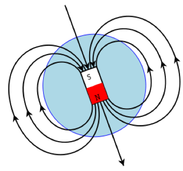
The magnetic fields are strongest at the north and south poles. The line in which a north pole would move in a field is referred to as the line of force of the magnetic field.

This magnetic field causes a force to be exerted on a current-carrying wire, but only when the field is perpendicular to the current. This force F = BIl where B is the magnetic flux density (T), I is the current (A) and l (m) is the length of the wire in contact with the magnetic field.  Furthermore, a current-carrying wire placed in a magnetic field will experience a force that acts perpendicular to the wire and to the lines of force of said magnetic field. However, a force will only be experienced if the wire is placed at a non-zero angle. This force will be highest when the wire is at right angles to the magnetic field, and zero when the wire is parallel.

Also, another way of looking at the field lines is that the line of force of a magnetic field is a line along which a free north pole would move in the field

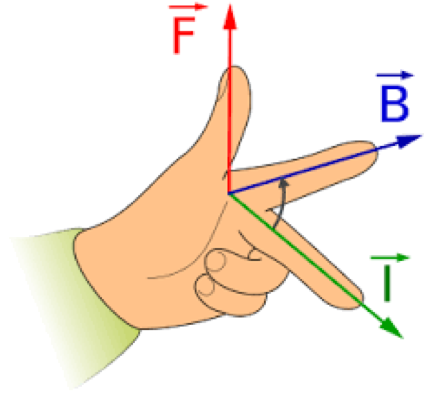
Fleming’s left hand rule

This rule can be used to determine the direction of current, of the magnetic field or of the force in a current-carrying wire. If two of the variables are known the third can be worked out using this rule. The rule clearly uses your left hand, where your thumb denotes motion, which also gives the direction of the force. The first finger represents the field direction and the second finger represents the direction of the current. You can remember it as the m in ‘thumb’ representing motion, the f in ‘first finger’ denoting field direction, and ‘second finger’ for current in the wire.

 

Fleming’s left hand rule is used for electric motors to describe something called the motor effect. It is used when dealing with situations involving the forces experienced by current carrying wires passing through a magnetic field.

Magnetic flux density B and definition of the tesla

Magnetic flux density, denoted by the symbol B can also be looked at as the magnetic field strength. It has the units Tesla (T). The direction of the force it exerts, and the direction of the field is found using Fleming’s left hand rule. The SI units of the Tesla are Nm^-1A^-1.

3.7.5.2 Moving charges in a magnetic field

Content

• Force on charged particles moving in a magnetic field, F = BQv when the field is perpendicular to velocity.
• Direction of force on positive and negative charged particles.
• Circular path of particles; application in devices such as the cyclotron

Force on charged particles moving in a magnetic field, F = BQv when the field is perpendicular to velocity.

In the last topic, the force experienced on a current-carrying wire in a magnetic field was studied, in this topic the force on charged particles moving in a magnetic field is the focus. The force can be calculated using the equation F = BQv, where B is the magnetic flux density (magnetic field strength), denoted by – (T), Q is the charge (C) and v is the velocity (ms^-1). However, this only stands true when the field is perpendicular to the velocity. An example is an electron beam fired through a vacuum tube, you can observe that in the presence of a magnetic field, the electrons will experience a force and be deflected in a certain direction.

Direction of force on positive and negative charged particles.

Fleming’s left hand rule can be used in this situation as well in order to work out the direction of the force on a moving charge. If the charge in question is an electron, then it is important to remember that the convention for the direction of flow of current is in the opposite direction to the direction of flow of the electrons. Therefore, the direction of force on positive and negative charged particles can be found using Fleming’s left hand rule.

Moreover, if you have a charge Q and –Q travelling in identical magnetic fields at the same speed, then F_Q = BQV and F_-Q = -BQV, so the force acts in the opposite direction.

Circular path of particles; application in devices such as the cyclotron

Magnetic fields can be used to control the path of beams of charged particles, for example in televisions. Since the force on a moving charged particle acts perpendicular to the direction of motion of the particle, a charged particle moving in a magnetic field will follow a circular path. Remembering back to circular motion, for a particle to maintain circular motion, its tangential velocity must act perpendicular to its direction of motion.

The consequences of this are that no work is done on the particle by the field as the force is always acting at right angles to the velocity. To exemplify this, W = Fd where d is the distance travelled in the direction of the force, however for a charged particle travelling in a magnetic field there is no movement in the direction of the force, so W = 0.

The radius of the path of the charged particles can be calculated by equating F = BQv and F = mv²/r. So you are left with BQv = mv²/r, which when rearranged for r gives r = mv/BQ.

An example of the application of magnetic fields is in a device called the cyclotron. This device produces high-energy beams that can be used in hospitals for treatments lie radiation therapy. Its structure is shown below, but essentially the cyclotron acts to accelerate particles.

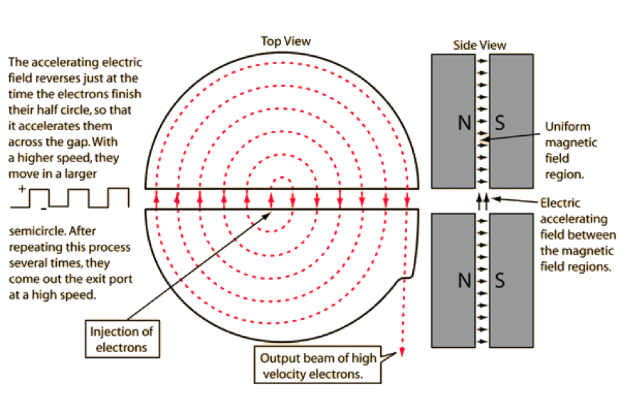
Charged particles enter the cyclotron at a site called a dee. Across the dees a high-frequency AC is applied, and a magnetic field is applied at right angles to the plane the dee is in. The particles within the cyclotron, usually electrons gain speed each time they pass from one dee to another, and so its radius increases. Once the radius is the same as the radius of the dee, the particle will leave the cyclotron.

Magnetic fields in mass spectrometry are also used in the analysis of the types of atoms present in a sample. The ions pass through velocity selectors that only allow an ion of a given velocity to pass. The velocity selector is comprised of a magnet and a pair of parallel plates. To find the velocity that is allowed to pass you must equate the force on the particle due to the magnetic field and the electric field. Therefore, VQ/d = BQv, so the accepted velocity is v = V/Bd. If the velocity is too high or too low, then the ion will either pass above or below the gap. Once the ion passes through the gap into the magnetic field, it will follow a path with a radius r = mv/BQ. This radius can be measured and so knowing the charge of the particle, the magnetic field strength and velocity of the particle, its mass can be calculated. This mass can then be used to identify the type of atoms present in a sample.

Jan 2010 Q22 Unit 4 Section A

Question:

An electron moves due North in a horizontal plane with uniform speed. It enters a uniform magnetic field directed due South in the same plane. Which one of the following statements concerning the motion of the electron in the magnetic field is correct?

1. It accelerated due West.
2. It slows down to zero speed and then accelerates due South.
3. It continues to move North with its original speed.
4. It is accelerated due North.

Answer:

If you draw a diagram of what is happening here, you will notice that the electron is moving parallel to the magnetic field.

As we already know, if a charge moves parallel to a magnetic field it will feel no force, so the answer is C.

3.7.5.3 Magnetic flux and flux linkage

Content

• Magnetic flux defined by F = BA, where B is normal to A
• Flux linkage as NΦ where N is the number of turns cutting the flux
• Flux and flux linkage passing through a rectangular coil rotated in a magnetic field
• Flux linkage NΦ = BANcosθ

Magnetic flux is defined by F = BA, where B is normal to A

Magnetic flux is defined as the total magnetic field which passes through a given area. It is calculated by using the equation F = BA, where F is magnetic flux with the units, Weber, denoted by the symbol – Wb. B is the magnetic field strength (T), and A is the area penetrated by the magnetic field(m²), which must be perpendicular to the magnetic field.

Flux linkage as NF where N is the number of turns cutting the flux

Flux linkage is denoted by NF, where N is the number of turns cutting the flux (cutting the magnetic field). T

Flux and flux linkage passing through a rectangular coil rotated in a magnetic field

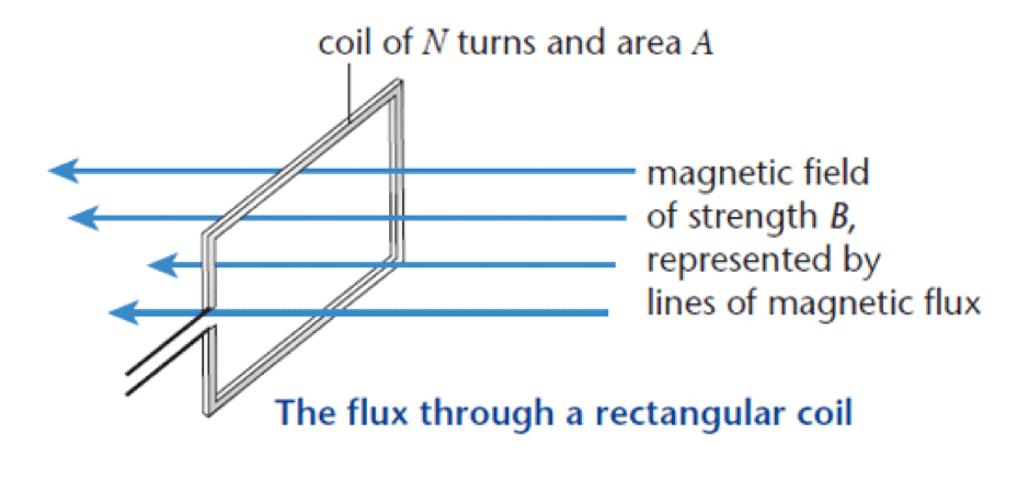
Source: https://revisionworld.com/a2-level-level-revision/physics/fields-0/electromagnetic-induction

The above diagram shows the flux and flux linkage through a rectangular coil in a magnetic field. Rotating the coil clockwise will result in less flux passing through the coil. This reduction of area in contact with the magnetic field will also reduce the flux linkage.

Flux linkage NΦ = BANcosθ

Flux linkage as mentioned before, is the magnetic flux linked to a coil. Also aforementioned, the flux linkage and flux passing through a coil will change as a result of rotating it in the magnetic field. This means that the overall flux linkage will decrease.

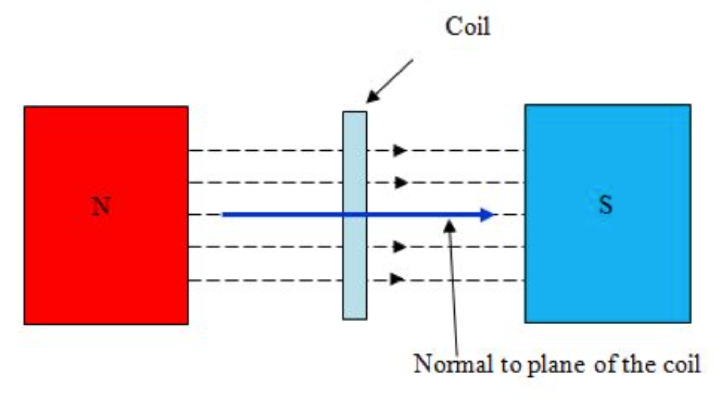
The magnetic field must be acting perpendicular to the area in the equation Φ = BA, so in calculating flux linkage, this condition must also be met. To meet this condition, you must find the angle between the normal to the coil, and magnetic field. The diagram below demonstrates this concept.

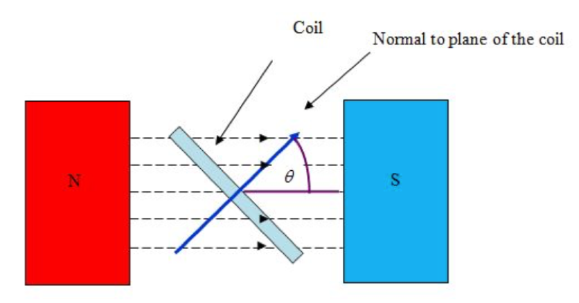
Source: http://www.antonine-education.co.uk/Pages/Physics_4/Magnetism/MAG_04/Mag_field_4.html

You will get the greatest value of flux linkage when cosθ = 1, ie θ = 0, thus a minimum at θ = 90.  At this minimum value, the field is parallel to the coil area, so no field lines pass through the coil area.

You can increase this value of flux linkage by increasing strength of the magnetic field. Or you can increase the ‘linked’ area. Another thing worth mentioning is that if you rotate a coil through 180°, the flux linkage is equal to –BAN.

3.7.5.4 Electromagnetic induction

Content

• Simple experimental phenomena.
• Faraday’s and Lenz’s laws.
• Magnitude of induced emf = rate of change of flux linkage e = NDF/Dt
• Applications such as a straight conductor moving in a magnetic field.
• Emf induced in a coil rotating uniformly in a magnetic field e =BANwsin(wt)

Simple experimental phenomena

Generating electricity can be done experimentally, using a magnet and a conducting wire. When the wire moves through the magnetic field, (or vice versa), and cuts the field line, an emf will be induced. If there is a complete circuit, then this emf will force a current to flow as electrons will be forced around the circuit. This effect is called electromagnetic induction. Moreover, to build on what I previously stated, if the wire moves parallel to the field lines, no emf will be induced.

Electromagnetic induction was discovered by Michael Faraday in 1832. It had been established that magnetic fields are produced in current-carrying wires, and Faraday wanted to know if you could use magnet to generate a current.

Other experiments to show this phenomenon can be done where the coil spins and magnet remains fixed, or the magnet spins and coil remains fixed. For example, in a dynamo.

• A dynamo is an electrical generator that works to convert mechanical energy into electrical energy. This is achieved by rotating a magnet within a coil of wire. When connected to a lamp, the rotation induces an emf, which causes a current to flow thus powering the lamp. The faster the rotation of the magnet, the greater the induced current and brighter the lights. This is utilised in bicycles that use this energy to power lamps.

The power is the work done per unit time. The induced emf multiplied by the current is equal to the rate of transfer of energy (power) from the source.

Faraday’s and Lenz’s laws.

Faraday’s law = “the induced emf in a circuit is equal to the rate of change of magnetic flux linkage through the circuit”.

Lenz’s law = “the direction of the induced current is always such that it opposes the change that causes the current”.

We already know that an emf is produced when a conducting wire is moved in a magnetic field. To be more precise, and according to Faraday’s law, this potential difference is produced as a result of a change in the motion. The induced voltage is dependent on the rate of change of magnetic flux linkage through a circuit.

This is represented by the equation e = NDF/Dt. Where e is the emf (V), N = number of turns, F is magnetic flux (Wb), and t is time (s). There should be a negative sign in front of the equation which is as a result of Lenz’s law, which will be covered next, which states the induced emf acts in such direction as to oppose the change that causes it.

If you have a set up of a coil connected to a meter measuring current, when a bar magnet is pushed into this coil, there will be a deflection on the meter. If you were to pull the magnet out of the coil in the opposite direction to that which it entered, the meter will deflect in the opposite direction.

We already know the definition of Lenz’s law: the diagram below shows its application.

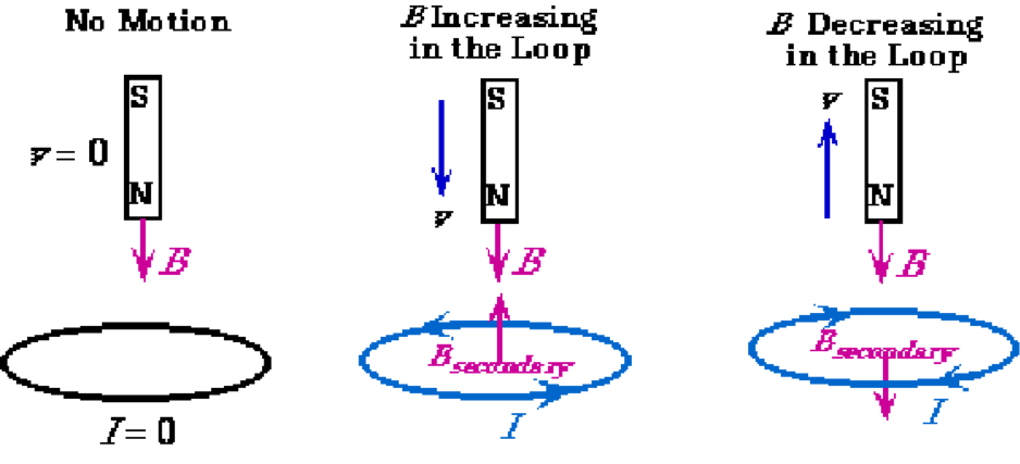
Source: https://astarmathsandphysics.com/ib-physics-notes/118-electricity/1271-lenz-s-law.html

When a permanently magnetised magnet passes through a coil that is connected to a meter there will be a deflection shown on the meter. This is because the coil of wire is seeing a changing magnetic field, thus a current is induced in the coil. This induced current creates a magnetic field in the coil that serves to oppose the incoming north pole (as shown above). It is important that this happens, because if it did not, energy, both electrical and kinetic would not be conserved. Energy would not be conserved as if the magnetic field supported the direction of movement of the magnet, then the north pole would be pulled in faster, which would increase the induced current and make the pole move in faster still. This would mean both kinetic energy and electrical energy would be created, thus not conserved.

The dynamo rule applies to electric generators, and is other-wise known as Fleming’s right hand rule. To remember that his right hand rule is for generators, you could use riGht-hand rule for Generators.

Also, to distinguish between using the left and right hand rules, you can remember that:

• For a motor the input energy is electrical energy and the useful output energy is mechanical energy.
• For a generator the input energy is mechanical energy and the useful output energy is electrical energy.

Generators vs Motors

The first diagram below shows an electric motor. In the motor a current is passed through the coil, generating a force on the coil and thus torque. This causes the rotational movement depicted in the image. This follows the point above that states electric motors use electrical energy as input energy, which is converted to useful mechanical output energy.

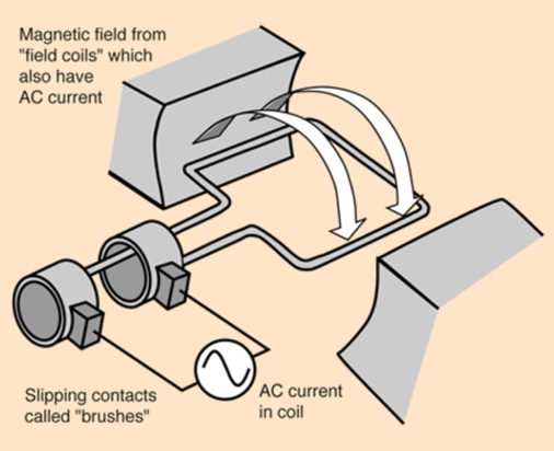
In an electric motor you will also get an emf is induced that will oppose the potential difference V applied to the motor, this in accordance with Lenz’s law. This then gives the equation V – ε = IR, as the back emf must be subtracted from the source pd. When the coil spins slowly, this induced emf is small thus current is high, and vice versa. Also, the equation V – ε = IR can be multiplied by I, to give VI – Iε = I²R. This tells you that the source power (VI) is equal to the power wasted due to resistance in the circuit added to the power transferred by the back emf.

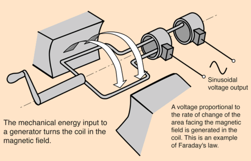
On the contrary, in generators the turning of the coils in the magnetic field produce emfs that force currents on both sides of the coil. The generated electrical energy can be described using Faraday’s Law of electromagnetic induction. Again, this follows the point above that stated useful mechanical energy is used to produce useful output electrical energy.

Magnitude of induced emf = rate of change of flux linkage ε = NΔΦ/Δt

This point has already been covered, and gives the equation for calculating the magnitude of the induced emf ε = NΔΦ/Δt. As also previously mentioned, this equation should actually have a negative sign at the beginning, as a result of Lenz’s Law.

Applications such as a straight conductor moving in a magnetic field.

An emf will be induced in a straight conductor moving in a magnetic field only if the conductor cuts the magnetic field lines.

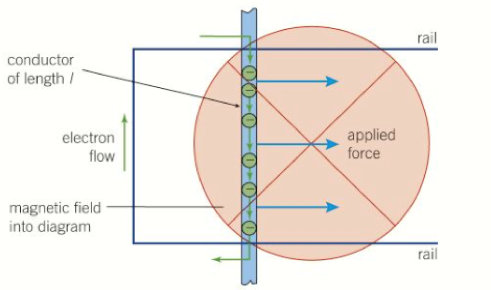
Source: Kerboodle A Level Physics Textbook

The diagram above shows a straight conductor moving in a magnetic field. The magnitude of the emf induced ε = E/Q, which can be used to derive Faradays’ equation. This equation tells us that the work done divided by the charge is equal to the induced emf.

We know that work done is equal to F x Δs, and we also know that the force on the conductor is F = BIl. Thus work done is equal to BIlΔs. We also know that the charge transferred is Q = IΔt.

The diagram above shows a straight conductor moving in a magnetic field. The magnitude of the emf induced ε = E/Q, which can be used to derive Faradays’ equation. This equation tells us that the work done divided by the charge is equal to the induced emf.

We know that work done is equal to F x Ds, and we also know that the force on the conductor is F = BIl. Thus work done is equal to BIlDs. We also know that the charge transferred is Q = IΔt.

So we can say that e = BIlΔs/IΔt = BlΔs/Δt. Also knowing that l x Δs is equal to the area swept out (length of the wire multiplied by distance moved by the wire), then we can write the induced emf e = BA/Δt, where BA equals magnetic flux (F). However, we also know that velocity = Δs/Δt, so it can also be said that ε = Blv, where B is the magnetic field strength, l is the length of the conductor, and v is the velocity of the conductor, all with their usual units.

There are other examples that can be used such as a fixed coil subject to a changing magnetic field. Or you could look at the example of a rectangular coil moving in a uniform magnetic field.

s, and we also know that the force on the conductor is F = BIl. Thus work done is equal to BIlΔs. We also know that the charge transferred is Q = IΔt.

So we can say that ε = BIlΔs/IΔt = BlΔs/Δt. Also knowing that l x Δs is equal to the area swept out (length of the wire multiplied by distance moved by the wire), then we can write the induced emf ε = BA/Δt, where BA equals magnetic flux (F). However, we also know that velocity = Δs/Δt, so it can also be said that ε = Blv, where B is the magnetic field strength, l is the length of the conductor, and v is the velocity of the conductor, all with their usual units.

There are other examples that can be used such as a fixed coil subject to a changing magnetic field. Or you could look at the example of a rectangular coil moving in a uniform magnetic field.

Emf induced in a coil rotating uniformly in a magnetic field ε =BANωsin(ωt)

In a simple AC generator, a rectangular coil is forced to spin in a magnetic field (as shown below). The coil sees a change in magnetic flux through it as it spins, generating an emf that drives the current. If the coils spin faster, at a higher frequency, ie there is a faster rate of change of flux, or there is a greater number of turns in the coil then the larger the peak emf will be. Also you could use a stronger magnet, or a bigger coil.

In this coil the angle is changing at the angular frequency ω, so the equation ωt would give you the angle between the normal to the area and the magnetic field lines at a given time. This means that the flux linkage NΦ = BANcos(ωt). It can be then shown mathematically that e =BANwsin(wt) by differentiating cos(ωt) with respect to time.

3.7.5.5 Alternating currents

Content

• Sinusoidal voltages and currents only; root mean square, peak and peak-to-peak values for sinusoidal waveforms only. 
• Application to the calculation of mains electricity peak and peak-to-peak voltage values.
• Use of an oscilloscope as a dc and ac voltmeter, to measure time intervals and frequencies, and to display ac waveforms.
• No details of the structure of the instrument are required but familiarity with the operation of the controls is expected.

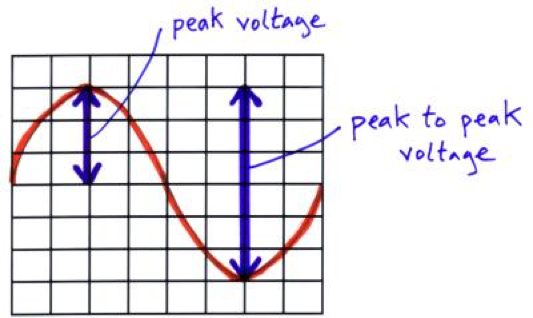
Sinusoidal voltages and currents only; root mean square, peak and peak-to-peak values for sinusoidal waveforms only

An alternating current is one in which the current is constantly changing direction. The rate at which these cycles occur per unit time (1s) is called the frequency. The frequency, f = 1/T, where T is time period (s). The units of frequency are hertz (Hz). The alternating currents studied in this specification are sinusoidal, ie can be modelled by sine waves. Since they can be modelled as sine waves, you can measure peak-to-peak values for the wave.

You can observe alternating currents by connecting a signal generator to an LED. If you make the frequency very low, you are able to see the lamp light up and fade out regularly. When the lamp lights up to its brightest, the peak value of the current is reached. This happens twice every cycle, when the current is at its peak value in either direction. The frequency is increased until the lamp flickers so fast that to the eye, there is no observable ‘flashing’, and it seems the intensity is constant.

Obviously an alternating current will produce an alternating power output, where this output will vary between 0 and I²R. For this alternating power output as shown below, there will be an average power output. If you took this average power output, and tried to find the corresponding constant current value that would give this power output value, you would find that the value is the root mean square of the alternating current, denoted by I_rms. So it can be said that ‘The root mean square value of an alternating current is the value of direct current that would give the same heating effect as the alternating current in the same resistor.’ The root mean square value is as it sounds, and is the root of the mean of the square of the original values.

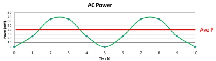
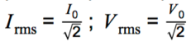
The rms value of both the current and potential difference can be calculated by multiplying the peak value (I₀/V₀) by 1/sqrt2.

Application to the calculation of mains electricity peak and peak-to-peak voltage values.

The UK mains electricity runs at about 230V, with a frequency of 50Hz. The peak to peak voltage of the mains supply is around 650V.

Source: http://physicsnet.co.uk/a-level-physics-as-a2/current-electricity/alternating-current-ac/

If we know the y-gain sensitivity of an oscilloscope, we are able to work out the peak to peak voltage. If the y-gain were set at 20V, then the peak to peak voltage would be 120V. Thus the peak voltage would be 60V, and from this the V_rms value could be calculated. We can then also find the peak current value.

Use of an oscilloscope as a dc and ac voltmeter, to measure time intervals and frequencies, and to display ac waveforms.

The point above illustrates how an oscilloscope can be used as an AC voltmeter. A DC signal would be a horizontal line, so the value of voltage can be calculated again, if the y gain is known. Time intervals between waveforms can be used to calculate the frequency of an AC supply.

No details of the structure of the instrument are required but familiarity with the operation of the controls is expected

3.7.5.6 The operation of a transformer

Content

• The transformer equation: N_S/N_P = V_S/V_P
• Transformer efficiency = I_SV_S/I_PV_P
• Production of eddy currents.
• Causes of inefficiencies in a transformer.
• Transmission of electrical power at high voltage including calculations of power loss in transmission lines.

The transformer equation: N_S/N_P = V_S/V_P

Alternating current is used widely for many reasons, for example it is easily produced by generators, the maximum voltage can be changed easily using a transformer, it can be controlled by a variety of different components, also it has a regular frequency which is useful for timing.

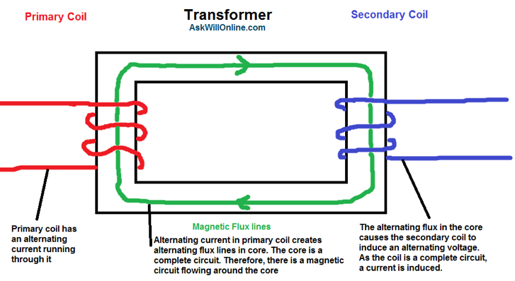
Transformers gain their name from their action, as they transform voltage and current from one level to another. Thus in transformers, the magnitude of the alternating current can be increased or decreased. The structure of a transformer comprises of a primary and a secondary coil linked by an iron core. The iron core serves to concentrate the magnetic field and can be magnetised/demagnetised easily to ‘transfer’ the magnetic field from one core to the other. Although, ‘transfer’ would not strictly be the most accurate term to use, but is useful for understanding the concept.

The action of a transformer is as follows: an alternating current is applied to the primary core and thus generates a constantly changing magnetic field in this core. This magnetic field then flows through the iron core.

Transformers can be step-up or step-down transformers, where step-up transformers step up the voltage and step down the current. The ratio of turns in the primary to the secondary coil determines whether the transformer is step-up or step-down.

• A step-up transformer has less turns on the primary coil, thus more on the secondary coil. This means the secondary voltage is increased from the primary voltage
• A step-down transformer has more turns on the primary coil, thus less turns on the secondary coil.

The equation N_S/N_P = V_S/V_P can be used to describe the action of transformers. N_S is the number of turns in the secondary coil and N_P is the number of turns in the primary coil. V_S is the voltage in the secondary coil, V_P is that in the primary coil. The equation is telling you that the ratio of output voltage to input voltage is equal to the ratio of turns of wire around the secondary coil, to the ratio of turns around the wire in the primary coil.

The diagram in the picture below gives a good outline of the action of a transformer. The transformer shown would not be a step-up or step-down transformer, as the number of turns on both sides is the same. This type of transformer can be used to restrict the amount of direct electrical connections, as the two coils are linked only via the magnetic field.

 

Transformer efficiency = I_SV_S/I_PV_P

To calculate the efficiency of a transformer you can use the equation above, where I_S is the secondary current, V_S is the secondary voltage. I_P is primary current and V_P the primary voltage. This equation is telling you that the efficiency of a transformer is the ratio of the power delivered by the secondary coil to the power supplied by the primary coil.

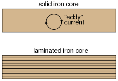
Production of eddy currents

Eddy currents are induced currents that are generated in the core itself. Iron is used for its ability to allow the magnetic field to flow in a circuit. However, it also conducts electricity, so there will be induced currents in the iron core itself, just like you get in the secondary coil.

These currents can be thought of as ‘swirling’ currents circulating perpendicular to the primary or secondary turns on the core. Their circular motion has given them a name that resembles ‘eddies’ in a stream of water that circulate as opposed to moving in a straight line. In the core, these eddies create induced magnetic fields that oppose the change of that of the original magnetic field, in accordance with Lenz’s law.

Causes of inefficiencies in a transformer.

1. Eddy currents. Iron is not as good a conductor of electricity as copper or aluminium, of which the coils are usually made. As a consequence, the eddy currents within the core receive a lot of resistance to their circulation. In overcoming this resistance, they dissipate power in the form of heat.
   1. Mitigation against these eddy currents involves using a laminated core as opposed to a solid iron core. Between each layer there is also a layer of insulation. The culmination of the insulation and separation of layers provides extra resistance to the eddy currents that are attempting to flow.

2. Resistance in the coils. More power will be dissipated in higher resistance coils, due to the heating effect of the current
   1. The coils are made of a material with a low resistance
3. Hysteresis in the core. The inclination to stay magnetised is called hysteresis, thus energy is used in overcoming this opposition to change each time the magnetic field produced in the primary coil changes polarity, ie 100 times a second from mains electricity (remember there are two peaks in a full AC cycle).
   1. To lessen these effects, a core with low hysteresis should be chosen. Essentially, a core that can be magnetised easily and demagnetised easily, like iron, should be used.

The inefficiencies within the transformer will usually increase in significance as the frequency is increased. As frequency increases, the effective resistance increases so more power is dissipated as heat from the windings. Within the magnetic core, losses will also increase as frequency increases, in terms of the eddy currents and hysteresis effects. Thus most large transformers have been designed so that they operate very efficiently across a very tiny array of frequencies.

Transmission of electrical power at high voltage including calculations of power loss in transmission lines.

In the UK, the national grid system is the supplier of electricity to most homes. The electricity is transmitted at high voltages, and then these voltages are stepped down so that they are safe to be transmitted into homes. Electrical power is more efficiently transferred at high voltages. This can be shown because P = VI, so for a given power output, P, the current required to reach the required power is decreased if voltage is increased. We already know that the current has a heating effect, so lower currents reduce this heating effect, thus reduce power dissipated (wasted) due to heating.

The current required to deliver this power output, P is given by the current, I = P/V. We also know that power is given by I²R, so if we want the power dissipated by the current, we can say that the power dissipated by the cables = I²R = P²R/V². If you were transmitting 10MW of power at 100kV through cables with a resistance of 200W, the current required would be 100A (P=VI). This power dissipated by this 100A current would therefore be 2MW. Thus higher voltages would be required as this power loss is quite significant.

AQA June 2011 Unit 4 Q5bii

Question:

Explain why the secondary windings of a step-down transformer should be made from thicker copper wire than the primary windings.

Answer:

• to reduce heating) loss [or energy/power/copper loss]
• (because) I_S > I_P
• and R is reduced (by use of thicker wire)